100-Days-Of-Machine-Learning
Table of Contents
- What is Machine Learning?
- AI vs ML vs DL
- Types of Machine Learning_
- Key differences between types of machine learning
- Batch Machine Learning vs Online Machine Learning
- Instance vs Model based learning
- Machine Learning Development Lifecycle
- What is a Tensor?
- Rank, Axis & Shape
1. What is Machine Learning?
Machine learning is a subset of artificial intelligence (AI) that focuses on teaching computers to learn from data and make predictions or decisions without being explicitly programmed to do so. It enables computers to learn patterns from data and utilize that knowledge to perform tasks or make predictions.
Explanation with Example
Imagine you want to build a program that can predict whether an email is spam or not spam (ham). Instead of manually writing rules to classify emails, you can use machine learning.
-
Data Collection: Gather a dataset of emails, each labeled as spam or not spam (ham).
-
Feature Extraction: Extract features from the emails, such as word frequency, presence of specific phrases, or email length.
-
Training Phase: Feed the labeled dataset into a machine learning algorithm. The algorithm learns from the data, identifying patterns that differentiate spam from non-spam emails.
-
Model Building: After training, the algorithm builds a model representing learned patterns. The model captures the relationship between email features and their labels (spam or not spam).
-
Prediction: When a new email arrives, input its features into the trained model. The model analyzes these features and predicts whether the email is spam or not based on learned patterns.
-
Evaluation and Improvement: Evaluate the model’s performance using a separate test dataset. Refine the model by adjusting parameters, using different algorithms, or gathering more data.
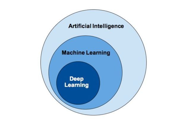
2. AI vs ML vs DL
| Aspect | Artificial Intelligence (AI) | Machine Learning (ML) | Deep Learning (DL) |
|---|---|---|---|
| Definition | AI is a broad field of computer science that aims to create machines or systems that can perform tasks that typically require human intelligence. | ML is a subset of AI that focuses on teaching computers to learn from data and make predictions or decisions without being explicitly programmed to do so. | DL is a subset of ML that uses neural networks with many layers (deep architectures) to learn from large amounts of data. |
| Scope | AI covers a wide range of techniques and applications, including problem-solving, natural language processing, robotics, computer vision, and more. | ML focuses specifically on algorithms and models that learn from data to perform tasks or make predictions. | DL specializes in training neural networks with multiple layers to automatically discover patterns and features from data. |
| Approach | In AI, various techniques are employed, including rule-based systems, expert systems, and statistical methods, to simulate human intelligence. | ML algorithms learn from data by identifying patterns and making predictions or decisions based on those patterns. | DL algorithms use deep neural networks, which consist of many layers of interconnected nodes, to automatically learn hierarchical representations of data. |
| Data Dependency | AI systems may or may not rely heavily on large amounts of data, depending on the specific application and approach used. | ML algorithms require labeled or unlabeled data for training to learn patterns and make predictions. The performance often improves with more high-quality data. | DL algorithms typically require large datasets for training, as they need vast amounts of data to effectively learn complex features and patterns. |
| Examples | Examples of AI include virtual assistants (like Siri or Alexa), self-driving cars, recommendation systems, and facial recognition systems. | Examples of ML applications include spam email detection, image recognition, language translation, and recommendation systems (like those used by Netflix or Amazon). | Examples of DL applications include image and speech recognition, natural language processing, autonomous vehicles, and medical diagnosis systems. |
In summary:
- AI is the broader field focused on creating intelligent systems.
- ML is a subset of AI that teaches computers to learn from data and make predictions or decisions.
- DL is a subset of ML that uses deep neural networks to learn from large amounts of data.
3. Types Of Machine Learning
- Supervised Learning:
- Supervised learning involves training a model on a labeled dataset, where each example in the dataset is paired with an input and an output label.
- The model learns to map inputs to outputs based on the examples provided during training.
- The goal is for the model to make predictions or decisions when presented with new, unseen data.
- Examples:
- Classification: Predicting a categorical label. For example, classifying emails as spam or not spam based on their content.
- Regression: Predicting a continuous value. For example, predicting the price of a house based on features like size, location, and number of bedrooms.
- Unsupervised Learning:
- Unsupervised learning involves training a model on an unlabeled dataset, where the model learns to find patterns or structure in the data without explicit guidance.
- The model discovers hidden patterns, groupings, or relationships within the data.
- There are no predefined output labels, and the model must find its own way to represent the data.
- Examples:
- Clustering: Grouping similar data points together. For example, clustering customers based on their purchasing behavior to identify market segments.
- Dimensionality Reduction: Reducing the number of features in a dataset while preserving its important characteristics. For example, reducing the dimensionality of high-dimensional data like images or text Blog.
- Association: Beer and Diapers: The Impossible Correlation Case Study
- Reinforcement Learning:
- Reinforcement learning involves training an agent to interact with an environment and learn the best actions to take to maximize some notion of cumulative reward.
- The agent learns through trial and error, receiving feedback in the form of rewards or penalties for its actions.
- The goal is to learn a policy—a mapping from states of the environment to actions—that maximizes the cumulative reward over time.
- Examples:
- Game Playing: Teaching an AI agent to play games like chess or Go Full Documentry on Go by Google DeepMind by rewarding good moves and penalizing bad ones.
- Robotics: Training a robot to perform tasks like navigating a maze or manipulating objects in the environment by rewarding successful actions.
4. Key differences between types of machine learning
| Aspect | Supervised Learning | Unsupervised Learning | Reinforcement Learning |
|---|---|---|---|
| Training Data | Labeled data | Unlabeled data | Agent-environment interaction with rewards/punishments |
| Learning Process | Learns from input-output pairs | Learns patterns or structure in data | Learns from feedback (rewards/penalties) for actions |
| Objective | Predict or classify new data | Discover hidden patterns or groupings | Learn optimal actions in an environment |
| Examples | Classification, Regression | Clustering, Dimensionality Reduction | Game playing, Robotics |
| Feedback Mechanism | Supervised (provided labels) | None (no explicit guidance) | Reward/Punishment based on actions |
| Goal | Minimize prediction error | Maximize data representation | Maximize cumulative reward over time |
In summary:
- Supervised Learning uses labeled data to predict or classify new data based on input-output pairs.
- Unsupervised Learning learns from unlabeled data to discover hidden patterns or structure in the data.
- Reinforcement Learning involves learning optimal actions through interaction with an environment, receiving feedback in the form of rewards or penalties.
5. Batch Machine Learning vs Online Machine Learning
### Batch Learning : Batch learning, also known as batch processing or offline learning, is a machine learning approach where the model is trained using the entire dataset at once. In batch learning, the algorithm processes the entire dataset, computes the gradients, and updates the model parameters all at once. Here’s a breakdown of batch learning:
- Data Processing:
- The entire dataset is loaded into memory and processed as a single batch.
- This means that all the data points, features, and labels are available to the algorithm simultaneously.
- Model Training:
- The model is trained on the entire dataset for multiple iterations or epochs.
- During each epoch, the algorithm goes through the entire dataset and updates the model parameters based on the computed gradients.
- Parameter Updates:
- After each epoch, the model’s parameters are updated based on the computed gradients of the entire dataset.
- This involves adjusting the weights and biases of the model to minimize the loss function, which measures the difference between the predicted outputs and the actual labels.
- Evaluation:
- Once the model has been trained, it is evaluated on a separate validation dataset to assess its performance.
- The model’s accuracy, precision, recall, or other relevant metrics are calculated to determine its effectiveness in making predictions on unseen data.
Advantages of Batch Learning:
- Simplicity: Batch learning is straightforward to implement and understand, making it suitable for beginners and for scenarios where simplicity is preferred.
- Stability: The model parameters are updated less frequently compared to online learning, resulting in stable learning and convergence.
Disadvantages of Batch Learning:
- Memory Intensive: Batch learning requires loading the entire dataset into memory, which can be challenging for large datasets that may not fit into memory.
- Lack of Adaptability: Batch learning is unable to adapt to changes in the data distribution without retraining the entire model, making it less suitable for dynamic or evolving datasets.
Batch learning is commonly used in scenarios where the entire dataset is available upfront, and real-time predictions are not required. It is well-suited for tasks such as offline data analysis, batch processing of large datasets, and model training in research and development environments.
Online Machine Learning
Online machine learning, also known as incremental learning or online learning, is a machine learning approach where the model is continuously updated with new data points as they become available. Unlike batch learning, where the model is trained using the entire dataset at once, online learning updates the model incrementally, typically on small batches or individual data points. Here’s an overview of online machine learning:
- Incremental Updates:
- In online learning, the model is updated continuously as new data points arrive.
- Instead of processing the entire dataset at once, the model processes incoming data points sequentially or in small batches.
- Training Approach:
- The model learns from new data points by updating its parameters incrementally.
- Each new data point or batch of data points is used to adjust the model’s parameters, such as weights and biases, to improve its performance.
- Adaptability:
- Online learning algorithms are more adaptable to changes in the data distribution over time.
- The model can quickly adjust to new patterns or trends in the data without requiring retraining on the entire dataset.
- Scalability:
- Online learning is suitable for handling large datasets that may not fit into memory or may be too computationally expensive to process at once.
- By processing data incrementally, online learning algorithms can efficiently scale to handle streaming data or continuous data streams.
- Real-time Predictions:
- Online learning allows for real-time predictions, as the model can update and make predictions on new data points as they arrive.
- This makes online learning suitable for applications that require immediate feedback or decision-making, such as fraud detection, recommendation systems, and online advertising.
Advantages of Online Learning:
- Adaptability: Online learning algorithms can adapt to changes in the data distribution over time, making them suitable for dynamic or evolving datasets.
- Scalability: Online learning is efficient for processing large datasets or streaming data, as it can handle data incrementally without requiring the entire dataset to be loaded into memory.
Disadvantages of Online Learning:
- Complexity: Online learning algorithms can be more complex to implement compared to batch learning, as they require handling data streams and managing model updates.
- Sensitivity to Noise: Online learning algorithms may be sensitive to noisy or irrelevant data points, requiring careful preprocessing and handling of data.
Online learning is commonly used in scenarios where data arrives continuously or in real-time, and where immediate feedback or predictions are required. It is well-suited for applications such as online advertising, recommendation systems, sensor data analysis, and anomaly detection.
6. Instance vs Model Based Learning
Instance-based learning and Model-based learning are two approaches in machine learning that differ in how they make predictions or decisions. Let’s explore each:
Instance-based Learning:
Instance-based learning, also known as memory-based learning or lazy learning, makes predictions based on the similarity between new data points and instances from the training dataset. It doesn’t explicitly build a model during the training phase. Instead, it stores all training instances and uses them to make predictions for new instances.
Here’s an overview:
- Training Phase:
- During training, instance-based learning algorithms simply memorize the training dataset, storing the instances and their corresponding labels.
- Prediction Phase:
- When a new instance is presented for prediction, the algorithm identifies the most similar instances from the training dataset (often using distance metrics such as Euclidean distance or cosine similarity).
- It then uses these similar instances to make a prediction for the new instance, typically by averaging or voting among the labels of the nearest neighbors.
- Examples:
- K-Nearest Neighbors (KNN): A popular instance-based learning algorithm that classifies new instances based on the majority class of their k nearest neighbors in the feature space.
- Case-based Reasoning (CBR): A problem-solving approach that retrieves similar past cases from memory and adapts them to solve new problems.
Advantages of Instance-based Learning:
- Simple to implement and understand.
- Capable of handling complex decision boundaries and non-linear relationships in the data.
Disadvantages of Instance-based Learning:
- Computationally expensive during prediction, especially for large datasets.
- Sensitive to irrelevant or noisy features in the dataset.
Model-based Learning:
Model-based learning involves building a model from the training data that captures the relationship between the input features and the output labels. The model is then used to make predictions for new, unseen data points.
Here’s an overview:
- Training Phase:
- During training, model-based learning algorithms use the training dataset to learn a model that best fits the data.
- This typically involves selecting a parametric form of the model (e.g., linear regression, decision tree, neural network) and optimizing its parameters to minimize a loss function.
- Prediction Phase:
- When a new instance is presented for prediction, the trained model is used to make predictions based on its learned parameters.
- The model applies the learned relationship between input features and output labels to generate predictions for new instances.
- Examples:
- Linear Regression: Fits a linear model to the training data to predict continuous output values.
- Decision Trees: Builds a tree-like structure to classify instances based on a series of decision rules learned from the training data.
Advantages of Model-based Learning:
- Efficient prediction phase, especially for large datasets, as the model is trained upfront.
- Generalizes well to unseen data if properly trained, capturing underlying patterns in the data.
Disadvantages of Model-based Learning:
- May not capture complex or non-linear relationships in the data without appropriate feature engineering or model complexity.
- Prone to overfitting if the model is too complex or the training dataset is too small.
In summary, instance-based learning makes predictions based on the similarity of new instances to past instances, while model-based learning builds a model from the training data to make predictions for new instances. Both approaches have their strengths and weaknesses and are suited for different types of problems and datasets.
7. Machine Learning Development Lifecycle (MLDLC)
- Gathering Data:
- In this initial phase, relevant data is collected from various sources such as databases, APIs, files, or sensors.
- The data collected should be comprehensive, representative, and of high quality to ensure the effectiveness of the machine learning model.
- Data gathering may involve acquiring labeled or unlabeled datasets, depending on the type of learning (supervised or unsupervised) being performed.
- Data Preparation:
- Once the data is collected, it needs to be prepared for analysis and modeling.
- This involves tasks such as cleaning the data to handle missing values, outliers, and inconsistencies, as well as formatting and transforming the data into a suitable format for analysis.
- Data preparation also includes splitting the dataset into training, validation, and test sets to evaluate the model’s performance.
- Data Wrangling:
- Data wrangling involves further preprocessing and transforming the data to extract meaningful insights and features.
- This may include feature engineering, where new features are created based on existing ones, as well as scaling, normalization, or encoding categorical variables.
- The goal of data wrangling is to improve the quality of the data and make it more suitable for model training.
- Analyze Data:
- In this phase, exploratory data analysis (EDA) is performed to gain a deeper understanding of the data and identify patterns, trends, and relationships.
- Visualization techniques such as histograms, scatter plots, and heatmaps are often used to visualize the data and uncover insights.
- The analysis of data helps inform decisions about feature selection, model selection, and potential areas for improvement.
- Train the Model:
- Once the data is prepared and analyzed, it’s time to train the machine learning model.
- This involves selecting an appropriate algorithm or model architecture based on the problem at hand and the characteristics of the data.
- The model is trained using the training dataset, where it learns patterns and relationships between the input features and the target variable.
- Training involves adjusting the model parameters to minimize a loss function, which measures the difference between the model’s predictions and the actual values.
- Test the Model:
- After training the model, it’s evaluated using the validation or test dataset to assess its performance.
- The model’s predictions are compared against the true values in the test set, and performance metrics such as accuracy, precision, recall, or F1-score are calculated.
- Testing helps ensure that the model generalizes well to unseen data and performs accurately in real-world scenarios.
- Deployment:
- Once the model has been trained and tested, it’s ready for deployment in production or real-world applications.
- Deployment involves integrating the model into existing systems or applications, where it can make predictions or decisions on new, unseen data.
- Monitoring and maintenance processes are put in place to continuously monitor the model’s performance, address any issues or drift, and update the model as needed to ensure its effectiveness over time.
The Machine Learning Lifecycle is iterative and may involve multiple iterations of model training, testing, and deployment as new data becomes available or business requirements evolve. Collaboration between data scientists, engineers, domain experts, and stakeholders is essential throughout the lifecycle to ensure the successful development and deployment of machine learning solutions.
8. What is a Tensor?
A tensor is a mathematical object representing a multi-dimensional array of numerical values. In the context of machine learning and deep learning, tensors are fundamental data structures used to represent and manipulate data. Tensors can have different numbers of dimensions, known as ranks, ranging from scalars (rank 0 tensors) to higher-dimensional arrays.
Types of Tensors and Their Explanation:
- Scalar (0D Tensor):
- A scalar is a single numerical value with no dimensions.
- It represents a single point in space.
- Example:
5
- Vector (1D Tensor):
- A vector is an array of numerical values arranged in a single dimension.
- It represents a sequence of values along a single axis.
- Example:
[1, 2, 3]
- Matrix (2D Tensor):
- A matrix is a 2-dimensional array of numerical values arranged in rows and columns.
- It represents a grid of values organized into rows and columns.
- Example:
[[1, 2, 3],
 [4, 5, 6]]
- Higher-dimensional Tensors (3D and above):
- Tensors with more than two dimensions, often used to represent complex data structures.
- They can represent data such as images, videos, or time-series data.
- Example:
[
  [[1, 2], [3, 4]],
  [[5, 6], [7, 8]],
  [[9, 10], [11, 12]]
]
Use Case Examples:
- Scalar (0D Tensor):
- Use Case: In deep learning, scalar tensors are commonly used to represent bias terms in neural network layers.
- Explanation: A scalar value is added to each neuron’s output in the layer, affecting the overall activation of the neuron.
- Vector (1D Tensor):
- Use Case: In sentiment analysis, a 1D tensor can represent the word embeddings of a sentence.
- Explanation: Each element of the vector corresponds to the embedding of a word in the sentence, capturing semantic information.
- Matrix (2D Tensor):
- Use Case: In image processing, a 2D tensor represents the pixel values of an image.
- Explanation: Each row of the matrix represents a row of pixels in the image, and each column represents a column of pixels.
- Higher-dimensional Tensors (3D and above):
- Use Case: In video classification, a 3D tensor can represent a sequence of video frames.
- Explanation: The first dimension represents time steps, the second and third dimensions represent the width and height of each frame, and the fourth dimension represents color channels.
Generalizing ND Tensor Code in Python:
Here’s a generalized function in Python to create an n-dimensional tensor using NumPy:
import numpy as np

def create_nd_tensor(shape):
    """
    Create an n-dimensional tensor with random values.

    Parameters:
    - shape: Tuple specifying the shape of the tensor.

    Returns:
    - nd_tensor: N-dimensional tensor with random values.
    """
    nd_tensor = np.random.rand(*shape)
    return nd_tensor

# Example usage:
shape = (2, 3, 4)  # Example shape for a 3D tensor
nd_tensor = create_nd_tensor(shape)
print("Generated", len(shape), "D tensor:")
print(nd_tensor)
print("Shape of the tensor:", nd_tensor.shape)
This function takes a tuple shape as input, specifying the dimensions of the desired tensor. It then generates random values to populate the tensor using NumPy’s np.random.rand function. Finally, it returns the created n-dimensional tensor.
9. Rank, Axis & Shape
- Rank:
- The rank of a tensor refers to the number of dimensions it has.
- For example, a scalar has rank 0, a vector has rank 1, a matrix has rank 2, and so on.
- In general, the rank of a tensor corresponds to the number of indices required to access its elements.
- Axis:
- Each dimension of a tensor is often referred to as an axis.
- For example, in a 2D tensor (matrix), the rows and columns correspond to the first and second axes, respectively.
- Axis indices are zero-based, meaning the first axis has index 0, the second axis has index 1, and so on.
- Shape:
- The shape of a tensor describes the size of each dimension.
- It is represented as a tuple of integers, where each integer specifies the size of the corresponding dimension.
- For example, a tensor with shape
(2, 3)has 2 rows and 3 columns. - The length of the shape tuple corresponds to the rank of the tensor.
In summary:
- Rank: Number of dimensions of a tensor.
- Axis: Each dimension of a tensor.
- Shape: Size of each dimension of a tensor, represented as a tuple.
Understanding these concepts is crucial for working with tensors in machine learning and deep learning, as they provide insights into the structure and organization of data within tensors.